Keywords

“Quality Content” and Where to Find It…

The first step toward quantifying something is to ask quantifying questions about it

What? How much? How many? How often?

These questions help form a narrative (what am I interested in?), and sell that narrative (why should I be interested?)

In essence, we are looking for good content, the “stuff” that is useful or interesting from the

Keywords

Let’s grab one of our course datasets: MTGJson, as documented in the appendix. If you’re following along, DVC can grab the data, as well: dvc import...

from tlp.data import DataLoader
df = DataLoader.mtg()

from tlp.data import mtg, styleprops_longtext

(df[['name', 'text','flavor_text']]
 .sample(10, random_state=2).fillna('').style
 .set_properties(**styleprops_longtext(['text','flavor_text']))
 .hide()
)

name	text	flavor_text
Saddleback Lagac	When Saddleback Lagac enters the battlefield, support 2. (Put a +1/+1 counter on each of up to two other target creatures.)	"A good lagac will carry you through thick and thin. A bad one . . . well, it's a tasty dinner." —Raff Slugeater, goblin shortcutter
Dragonskull Summit	Dragonskull Summit enters the battlefield tapped unless you control a Swamp or a Mountain. {T}: Add {B} or {R}.	When the Planeswalker Angrath called dinosaurs "dragons," the name stuck in certain pirate circles.
Snow-Covered Forest	({T}: Add {G}.)
Earthshaker Giant	Trample When Earthshaker Giant enters the battlefield, other creatures you control get +3/+3 and gain trample until end of turn.	"Come, my wild children. Let's give the interlopers a woodland welcome."
Howlpack Piper // Wildsong Howler	This spell can't be countered. {1}{G}, {T}: You may put a creature card from your hand onto the battlefield. If it's a Wolf or Werewolf, untap Howlpack Piper. Activate only as a sorcery. Daybound (If a player casts no spells during their own turn, it becomes night next turn.)
Frost Bite	Frost Bite deals 2 damage to target creature or planeswalker. If you control three or more snow permanents, it deals 3 damage instead.	"Don't wander far—it's a bit nippy out there!" —Leidurr, expedition leader
Sisay's Ring	{T}: Add {C}{C}.	"With this ring, you have friends in worlds you've never heard of." —Sisay, Captain of the *Weatherlight*
Spectral Bears	Whenever Spectral Bears attacks, if defending player controls no black nontoken permanents, it doesn't untap during your next untap step.	"I hear there are bears—or spirits—that guard caravans passing through the forest." —Gulsen, abbey matron
Mardu Hateblade	{B}: Mardu Hateblade gains deathtouch until end of turn. (Any amount of damage it deals to a creature is enough to destroy it.)	"There may be little honor in my tactics, but there is no honor in losing."
Forest	({T}: Add {G}.)

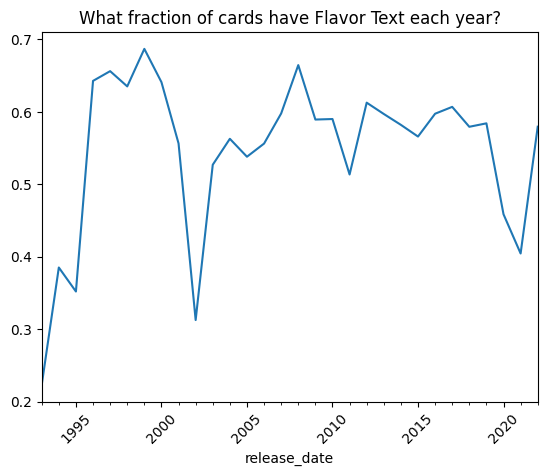
Flavor text has been a staple of Magic cards for a long time. A lot of players gravitate to it, even more than the game itself.

There are easter-eggs, long-running gags, and returning characters. Flavor text is really cool.

That sounds like some interesting “content”…what is its history?

{figure-md} feeling-lost

Magic: The Gathering can be a lot to take in, and it’s easy to get lost in all the strange words. This is why we use it for TLP! Thankfully, us “lost” folks have a mascot, in old Fblthp, here!

import pandas as pd
import numpy as np
import hvplot.pandas
(df
 .set_index('release_date')
 .sort_index()
 .resample('Y')
 .apply(lambda grp: grp.flavor_text.notna().sum()/grp.shape[0])
#  .apply(lambda grp: )
).plot( rot=45, title='What fraction of cards have Flavor Text each year?')

<Axes: title={'center': 'What fraction of cards have Flavor Text each year?'}, xlabel='release_date'>

There’s a lot of other data avaliable, as well!

mtg.style_table(df.sample(10, random_state=2),
                        hide_columns=['text','flavor_text'])

color_identity	colors	converted_mana_cost	edhrec_rank	keywords	mana_cost	name	number	power	rarity	subtypes	supertypes	text	toughness	types	flavor_text	life	code	release_date	block
		4	16804	['Support']		Saddleback Lagac	18	3	common	['Lizard']	[]	When Saddleback Lagac enters the battlefield, support 2. (Put a +1/+1 counter on each of up to two other target creatures.)	1	['Creature']	"A good lagac will carry you through thick and thin. A bad one . . . well, it's a tasty dinner." —Raff Slugeater, goblin shortcutter	nan	DDR	Sep '16	None
		0	125	None		Dragonskull Summit	252	nan	rare	[]	[]	Dragonskull Summit enters the battlefield tapped unless you control a Swamp or a Mountain. {T}: Add {B} or {R}.	nan	['Land']	When the Planeswalker Angrath called dinosaurs "dragons," the name stuck in certain pirate circles.	nan	XLN	Sep '17	Ixalan
		0	nan	None		Snow-Covered Forest	254	nan	common	['Forest']	['Basic' 'Snow']	({T}: Add {G}.)	nan	['Land']		nan	MH1	Jun '19	None
		6	9001	['Trample']		Earthshaker Giant	5	6	nan	['Giant' 'Druid']	[]	Trample When Earthshaker Giant enters the battlefield, other creatures you control get +3/+3 and gain trample until end of turn.	6	['Creature']	"Come, my wild children. Let's give the interlopers a woodland welcome."	nan	GN2	Nov '19	None
		4	7392	['Daybound']		Howlpack Piper // Wildsong Howler	392	2	rare	['Human' 'Werewolf']	[]	This spell can't be countered. {1}{G}, {T}: You may put a creature card from your hand onto the battlefield. If it's a Wolf or Werewolf, untap Howlpack Piper. Activate only as a sorcery. Daybound (If a player casts no spells during their own turn, it becomes night next turn.)	2	['Creature']		nan	VOW	Nov '21	Innistrad: Double Feature
		1	11917	None		Frost Bite	404	nan	common	[]	['Snow']	Frost Bite deals 2 damage to target creature or planeswalker. If you control three or more snow permanents, it deals 3 damage instead.	nan	['Instant']	"Don't wander far—it's a bit nippy out there!" —Leidurr, expedition leader	nan	KHM	Feb '21	None
		4	2463	None		Sisay's Ring	154	nan	common	[]	[]	{T}: Add {C}{C}.	nan	['Artifact']	"With this ring, you have friends in worlds you've never heard of." —Sisay, Captain of the *Weatherlight*	nan	VIS	Feb '97	Mirage
		2	8173	None		Spectral Bears	131	3	uncommon	['Bear' 'Spirit']	[]	Whenever Spectral Bears attacks, if defending player controls no black nontoken permanents, it doesn't untap during your next untap step.	3	['Creature']	"I hear there are bears—or spirits—that guard caravans passing through the forest." —Gulsen, abbey matron	nan	ME1	Sep '07	None
		1	17021	None		Mardu Hateblade	16	1	common	['Human' 'Warrior']	[]	{B}: Mardu Hateblade gains deathtouch until end of turn. (Any amount of damage it deals to a creature is enough to destroy it.)	1	['Creature']	"There may be little honor in my tactics, but there is no honor in losing."	nan	KTK	Sep '14	Khans of Tarkir
		0	nan	None		Forest	247	nan	common	['Forest']	['Basic']	({T}: Add {G}.)	nan	['Land']		nan	M11	Jul '10	Core Set

import matplotlib.pyplot as plt

def value_ct_wordcloud(s: pd.Series):
    from wordcloud import WordCloud
    wc = (WordCloud(background_color="white", max_words=50)
          .generate_from_frequencies(s.to_dict()))
    plt.figure()
    plt.imshow(wc, interpolation="bilinear")
    plt.axis("off")
    plt.show()

(df.types.explode().value_counts()
 .pipe(value_ct_wordcloud)
)

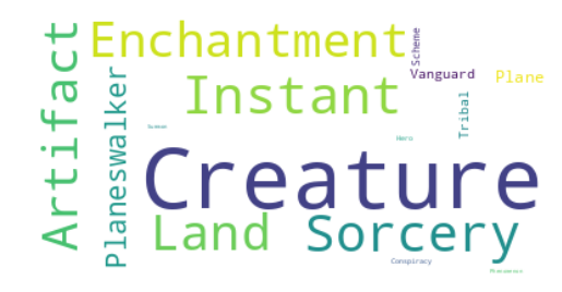
What “types” of cards are there? What are the “subtypes” of cards, and how are they differentiate from “types”?

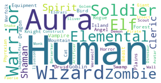
It looks like this magic is quite anthropocentric!

(df.subtypes.explode().value_counts()
 .pipe(value_ct_wordcloud) 
)
# df.subtypes.value_counts()

Keywords

These kinds of comma-separated lists of “content-of interest” are generally called keywords. Here, we have been told what those keywords are, which is nice!

Question… would we always have been able to find them from the text?

def plot_textual_occurrence(
    df,
    key_col='keywords', 
    txt_col='text',
    pre = str # do nothing, make str
): 

    def keyword_in_txt(df_row):
        return (
            pre(df_row[key_col]) 
            in 
            pre(df_row[txt_col])
        )

    return (
        df[['text','keywords']].explode('keywords')
        .dropna(subset=['keywords'])
        .assign(
            textual=lambda df: 
            df.apply(keyword_in_txt, axis=1)
        )
        .groupby('keywords')['textual'].mean()
        .sort_values()
        .head(40)
        .hvplot.barh(
            title='Fraction of text containing keyword',
            frame_width=250, 
            frame_height=350
        )
    )

plot_textual_occurrence(df)

# wait...let's lowercase
plot_textual_occurrence(
    df, pre=lambda s: str(s).lower()
)

Recap

• Content in a document can occur in or alongside the text itself.

• Keywords are individual markers of useful content, often comma-separated

• Often you need to “tidy up” keyword lists with df.explode('my_keyword_column)

• Keywords can be supplied a priori (by experts, etc.) Use them!

• Supplied keywords have become divorced from the text… do they match?

Sanity-check

So:

• interesting content \(\rightarrow\) frequent content

  \(\rightarrow\) frequent keywords

What assumption(s) did we make just then?

• interesting content \(\rightarrow\) frequent content \(\rightarrow\) frequent keywords

What are words?

We are assuming that a “fundamental unit” of interesting content is a “word”. Remember, though, that a “word” is not a known concept to the computer… all it knows are “strings”

Individual characters, or even slices of strings (i.e. substrings) don’t have any specific meaning to us as concepts (directly). This means there is a fundamental disconnect (and, therefore, a need for translation) between strings and words, to allow the assumption above to work in the first place.

%%coconut
def substrings(size) = 
    """return a function that splits stuff into 'size'-chunks and prints as list"""
    groupsof$(size)..> map$(''.join) ..> list ..> print

my_str = "The quick brown fox"
my_str |> substrings(3)
my_str |> substrings(4)
my_str |> substrings(5)

['The', ' qu', 'ick', ' br', 'own', ' fo', 'x']

['The ', 'quic', 'k br', 'own ', 'fox']

['The q', 'uick ', 'brown', ' fox']

Only some of these would make sense as “words”, and that’s only if we do some post-processing in our minds (e.g. own could be a word, but is that the same as [ ]own?

How do we:

• formalize turning strings into the these concept-compatible “word” objects?

• Apply this to our text, so we know the concepts available to us?

Intro to Tokenization

Preferably, we want to replace the substrings function with something that looked like:

substr(my_str)
>>> ['The', 'quick', 'brown', 'fox']

In text-processing, we have names for these units of text that communicate a single concept: tokens. The process of breaking strings of text into tokens is called tokenization.

There’s actually a few special words we use in text analysis to refer to meaningful parts of our text, so let’s go ahead and define them ([]):

corpus

the set of all text we are processing

e.g. the text from entire MTGJSON dataset is our corpus

document

a unit of text forming an “observation” that we can e.g. compare to others

e.g. each card in MTGJSON is a “document” containing a couple sections of text

token

a piece of text that stands for a word.

the flavor-text for Mardu Hateblade: has 15 tokens, excluding punctuation:

“There may be little honor in my tactics, but there is no honor in losing.”

types

unique words in the vocabulary

For the same card above, there are 15 tokens, but only 13 types (therex2, honor x2, in x2)

Using Pandas’ .str

There are a number of very helpful tools in the pandas .str namespace of the Series object. We can return to our card example from before:

card = df[df.name.str.fullmatch('Mardu Hateblade')]
flav = card.flavor_text
print(f'{card.name.values}:\n\t {flav.values[0]}')
# df.iloc[51411].flavor_text

['Mardu Hateblade']:
	 "There may be little honor in my tactics, but there is no honor in losing."

flav.str.upper()  # upper-case

24660    "THERE MAY BE LITTLE HONOR IN MY TACTICS, BUT ...
Name: flavor_text, dtype: string

flav.str.len()  # how long is the string?

24660    75
Name: flavor_text, dtype: Int64

verify: the number of tokens and types

# Should be able to split by the spaces...
print(flav.str.split(' '), '\n')
print("no. tokens: ", flav.str.split(' ').explode().size)
print("no. types: ",len(flav.str.split(' ').explode().unique()))

24660    ["There, may, be, little, honor, in, my, tacti...
Name: flavor_text, dtype: object

no. tokens: 

15

no. types: 

13

wait a minute…

flav.str.split().explode().value_counts()

flavor_text
honor       2
in          2
"There      1
may         1
be          1
little      1
my          1
tactics,    1
but         1
there       1
is          1
no          1
losing."    1
Name: count, dtype: int64

This isn’t right!

We probably want to split on anything that’s not “letters”:

flav.str.split('[^A-Za-z]').explode().value_counts()

flavor_text
           4
honor      2
in         2
There      1
may        1
be         1
little     1
my         1
tactics    1
but        1
there      1
is         1
no         1
losing     1
Name: count, dtype: int64

Much better!

So what is this devilry? This [^A-Za-z] is a pattern — a regular expression — for “things that are not alphabetical characters in upper or lower-case”. Powerful, right? We’ll cover this in more detail in the next section.

In the meantime, let’s take a look again at this workflow pattern:

tokenize \(\rightarrow\) explode

Tidy Text

but first…

Tidy Data Review

Let’s review an incredibly powerful idea from the R community: using tidy data.

Tidy data is a paradigm to frame your tabular data representation in a consistent and ergonomic way that supports rapid manipulation, visualization, and cleaning. Imagine we had this non-text dataset (from Hadley Wickham’s paper Tidy Data):

df_untidy = pd.DataFrame(index=pd.Index(name='name', data=['John Smith', 'Jane Doe', 'Mary Johnson']), 
             data={'treatment_a':[np.nan, 16, 3], 'treatment_b': [2,11,1]})
df_untidy

	treatment_a	treatment_b
name
John Smith	NaN	2
Jane Doe	16.0	11
Mary Johnson	3.0	1

We could also represent it another way:

df_untidy.T

name	John Smith	Jane Doe	Mary Johnson
treatment_a	NaN	16.0	3.0
treatment_b	2.0	11.0	1.0

I’m sure these might be equally likely to see in someone’s excel sheet, entering this data. But, say we want to visualize this table? Or start comparing each of the cases? This is going to take a lot of manipulation every time we want a different thing.

For data to be Tidy Data, we need 3 things:

1. Each variable forms a column.

2. Each observation forms a row.

3. Each type of observational unit forms a table.

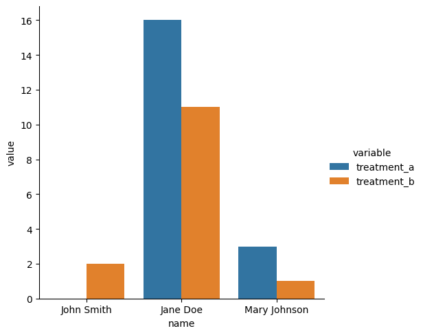
df_tidy = df_untidy.reset_index().melt(id_vars=['name'])
df_tidy

	name	variable	value
0	John Smith	treatment_a	NaN
1	Jane Doe	treatment_a	16.0
2	Mary Johnson	treatment_a	3.0
3	John Smith	treatment_b	2.0
4	Jane Doe	treatment_b	11.0
5	Mary Johnson	treatment_b	1.0

Suddenly things like comparing, plotting, and counting become trivial with simple table operations.

But doesn’t this waste table space? It’s so much less compact!

That’s excel talking! The “wasted space” is incredibly negligible at this scale, compared to the ergonomic benefit of representing your data long-form, with one-observation-per-row. Now you get exactly one column for every variable, and one row for every point of data, making your manipulations much cleaner.

import seaborn as sns
sns.catplot(
    data=df_tidy, 
    y='value', 
    x='name', 
    hue='variable', # try commenting/changing to 'col'!
    kind='bar'
)

<seaborn.axisgrid.FacetGrid at 0x7fa5f2045c30>

Back to Tidy Text

So, hang on, aren’t documents our observational-level? Wouldn’t that make e.g. the MTGJSON dataset already “tidy”??

Yes!

But only if we are observing cards, which, for things like release date or mana cost, maybe that’s true.

Instead, we are trying to find (observe) the occurrences of “interesting content”, which we broke down into tokens.

We thus define the tidy text format as being a table with one-token-per-row. A token is a meaningful unit of text, such as a word, that we are interested in using for analysis, and tokenization is the process of splitting text into tokens. This one-token-per-row structure is in contrast to the ways text is often stored in current analyses, perhaps as strings or in a document-term matrix.

%%coconut
import nltk
import janitor as pj
nltk.download('punkt')

tidy_df = (
    df
    .add_column('word', wordlists)
    .also(df -> print(df.word.head(10)))
    .explode('word')
    .rename_axis('card_id')
    .reset_index()
) where: 
    wordlists = (
        df.flavor_text
        .fillna('')
        .str.lower()
        .apply(nltk.tokenize.word_tokenize)
    )

[nltk_data] Downloading package punkt to /home/tbsexton/nltk_data...

[nltk_data]   Package punkt is already up-to-date!

0                                                   []
1    [every, tear, shed, is, a, drop, of, immortali...
2                                                   []
3    [the, perfect, antidote, for, a, tightly, pack...
4    [life, is, measured, in, inches, ., to, a, hea...
5    [the, cave, floods, with, light, ., a, thousan...
6    [``, we, called, them, 'armored, lightning, .,...
7    [``, we, called, them, 'armored, lightning, .,...
8    [``, mercadia, 's, masks, can, no, longer, hid...
9    [``, no, doubt, the, arbiters, would, put, you...
Name: word, dtype: object

tidy_df.word.value_counts().head(20)

word
.        38331
the      30973
,        23947
of       14566
''       14079
``       13951
to       10857
a         9839
and       7563
is        6111
it        5895
in        5636
's        4994
i         4053
you       3877
for       3541
as        3185
are       2921
that      2921
their     2644
Name: count, dtype: int64

Assumption Review

Words? Stopwords.

The “anti-keyword”

Stuff that we say, a priori is uninteresting. Usually articles, pasive being verbs, etc.

nltk.download('stopwords')
stopwords = pd.Series(name='word', data=nltk.corpus.stopwords.words('english'))
print(stopwords.tolist())

[nltk_data] Downloading package stopwords to
[nltk_data]     /home/tbsexton/nltk_data...

[nltk_data]   Package stopwords is already up-to-date!

['i', 'me', 'my', 'myself', 'we', 'our', 'ours', 'ourselves', 'you', "you're", "you've", "you'll", "you'd", 'your', 'yours', 'yourself', 'yourselves', 'he', 'him', 'his', 'himself', 'she', "she's", 'her', 'hers', 'herself', 'it', "it's", 'its', 'itself', 'they', 'them', 'their', 'theirs', 'themselves', 'what', 'which', 'who', 'whom', 'this', 'that', "that'll", 'these', 'those', 'am', 'is', 'are', 'was', 'were', 'be', 'been', 'being', 'have', 'has', 'had', 'having', 'do', 'does', 'did', 'doing', 'a', 'an', 'the', 'and', 'but', 'if', 'or', 'because', 'as', 'until', 'while', 'of', 'at', 'by', 'for', 'with', 'about', 'against', 'between', 'into', 'through', 'during', 'before', 'after', 'above', 'below', 'to', 'from', 'up', 'down', 'in', 'out', 'on', 'off', 'over', 'under', 'again', 'further', 'then', 'once', 'here', 'there', 'when', 'where', 'why', 'how', 'all', 'any', 'both', 'each', 'few', 'more', 'most', 'other', 'some', 'such', 'no', 'nor', 'not', 'only', 'own', 'same', 'so', 'than', 'too', 'very', 's', 't', 'can', 'will', 'just', 'don', "don't", 'should', "should've", 'now', 'd', 'll', 'm', 'o', 're', 've', 'y', 'ain', 'aren', "aren't", 'couldn', "couldn't", 'didn', "didn't", 'doesn', "doesn't", 'hadn', "hadn't", 'hasn', "hasn't", 'haven', "haven't", 'isn', "isn't", 'ma', 'mightn', "mightn't", 'mustn', "mustn't", 'needn', "needn't", 'shan', "shan't", 'shouldn', "shouldn't", 'wasn', "wasn't", 'weren', "weren't", 'won', "won't", 'wouldn', "wouldn't"]

NB

Discussion: stopwords are very context-sensitive decisions.

• Can you think of times when these are not good stop words?

• When would these terms actually imply interesting “content”?

(tidy_df
 .filter_column_isin(
     'word',
     nltk.corpus.stopwords.words('english'), 
     complement=True # so, NOT IN
 )
 .word.value_counts().head(30)
)

word
.         38331
,         23947
''        14079
``        13951
's         4994
*          2106
one        1799
n't        1741
?          1529
!          1382
never       980
life        956
like        926
death       902
world       834
every       828
even        821
would       707
time        699
power       677
'           660
see         651
:           643
us          625
must        613
know        609
many        552
first       547
could       535
always      532
Name: count, dtype: int64

This seems to have worked ok.

Now we can see some interesting “content” in terms like “life”, “death”, “world”, “time”, “power”, etc.

What might we learn from these keywords? What else could we do to investigate them?

Importance \(\approx\) Frequency?

%%coconut 
keywords = (
    tidy_df
    .assign(**{
        'year': df -> df.release_date.dt.year,
        'yearly_cnts': df -> df.groupby(['year', 'word']).word.transform('count'),
        'yearly_frac': df -> df.groupby('year').yearly_cnts.transform(grp->grp/grp.count().sum())
    })
    .filter_column_isin(
        'word', 
        ['life', 'death']
#         ['fire', 'water']
    )
)

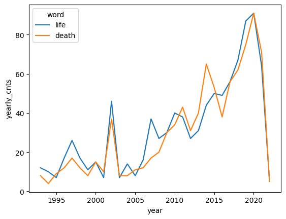
sns.lineplot(data=keywords, x='year', y='yearly_cnts',hue='word')

<Axes: xlabel='year', ylabel='yearly_cnts'>

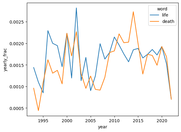
sns.lineplot(data=keywords, x='year', y='yearly_frac',hue='word')

<Axes: xlabel='year', ylabel='yearly_frac'>

Lessons:

• Frequency can have many causes, few of which correlate to underlying “importance”

• Starting to measure importance? relative comparisons, ranked.

This get’s us part of the way toward information-theoretic measures, and other common weighting schemes. More to come in the Measure & Evaluate chapter.

Aside: how many keywords in my corpus?

token

a piece of text that stands for a word.

types

unique words in the vocabulary

So:

• num. types is the size of the vocabulary \(\|V\|\)

• num. tokens is the size of the corpus \(\|N\|\)

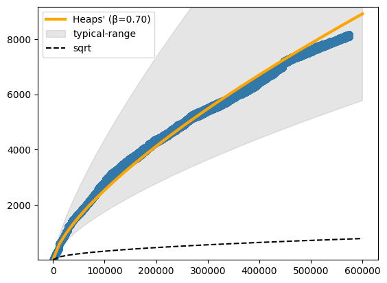
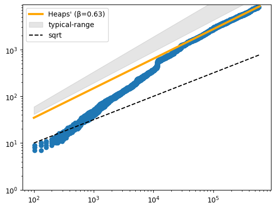
Heap’s Law: $\( \|V\| = k\|N\|^\beta\)$

rand = np.random.default_rng()
def sample_docs(df, id_col='card_id', shuffles=5, rng=np.random.default_rng()):
    samps = []
    for i in range(shuffles):
        shuff = df.shuffle()
        samps+=[pd.DataFrame({
            'N': shuff.groupby(id_col).word.size().cumsum(), 
            'V': (~shuff.word.duplicated()).cumsum()
        })]
    return pd.concat(samps).reset_index(drop=True).dropna().query('N>=100')

heaps = sample_docs(tidy_df)
heaps

	N	V
8	103.0	9
9	132.0	10
10	160.0	11
11	197.0	12
12	212.0	13
...	...	...
2353349	574218.0	8170
2353350	574244.0	8170
2353351	574245.0	8170
2353352	574246.0	8170
2353353	574247.0	8170

281790 rows × 2 columns

from scipy.optimize import curve_fit
def heaps_law(n, k, beta): 
    return k*n**beta

def fit_heaps(data, linearize=False):
    if not linearize:
        params, _ = curve_fit(
            heaps_law,
            data.N.values, 
            data.V.values
        )
    else: 
        log_data = np.log(data)
        params, _ = curve_fit(
            lambda log_n, k, beta: np.log(k) + beta*log_n,
            log_data.N.values,
            log_data.V.values
        )
    return params

def plot_heaps_law(heaps, log_scale=False, linearize=False):
    params = fit_heaps(heaps, linearize=linearize)
    print(f'fit: k={params[0]:.2f}\tβ={params[1]:.2f}\tlinear-fit={linearize}')
    plt.figure()
    x = np.linspace(100,6e5)
    plt.scatter(heaps.N, heaps.V, )
    plt.plot(
        x, 
        heaps_law(x, params[0], params[1]), 
        color='orange', lw=3, label=f'Heaps\' (β={params[1]:.2f})'
    )
    plt.fill_between(x, 
                     heaps_law(x, params[0], 0.67),
                     heaps_law(x, params[0], 0.75),
                    color='grey', alpha=.2, 
                    label='typical-range')

    plt.ylim(1,heaps.V.max()+1000)
    plt.plot(x, np.sqrt(x), ls='--', label='sqrt', color='k')
    if log_scale:
        plt.xscale('log')
        plt.yscale('log')
    plt.legend()
plot_heaps_law(heaps)

fit: k=1.89	β=0.63	linear-fit=False

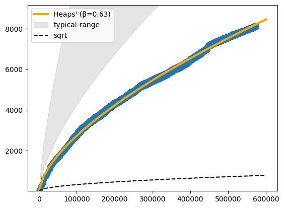
So, our data grows in complexity a lot faster than the square-root of it’s size, but slower than “typical” text.

Most data-sets in NLP are between 0.67-0.75, so we

• get a lot of complexity early on, but …

• there’s not such an extended amout of “new concepts” to find, after a while.

Pretty typical of “technical”, or, synthetic and domain-centric language. Lot’s of variety initially, but limited in scope compared to casual speech.

plot_heaps_law(heaps, log_scale=True)

fit: k=1.89	β=0.63	linear-fit=False

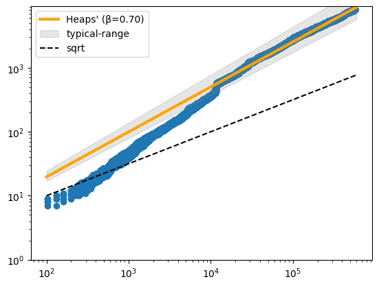
plot_heaps_law(heaps, log_scale=True, 
               linearize=True)

fit: k=0.78	β=0.70	linear-fit=True

plot_heaps_law(heaps, log_scale=False, linearize=True)

fit: k=0.78	β=0.70	linear-fit=True